Basic example
In this example, we showcase the use of pyshqg:
we first show how to check that the integration unit test is satisfied;
then we show how to compute a model trajectory;
finally we show how to plot the final state of the trajectory.
Let us start by importing numpy and pyshqg. Note that in pyshqg we only import what we will actually use.
[1]:
import numpy as np
from pyshqg.backend.numpy_backend import NumpyBackend as Backend
from pyshqg.core.constructors import construct_model, construct_integrator
from pyshqg.preprocessing.reference_data import load_test_data
Unit test
Let us define a function to compute the relative root mean squared error (RMSE) between two vectors.
[2]:
def relative_rmse(x, y):
    rms_x = np.sqrt(np.mean(np.square(x)))
    rms_y = np.sqrt(np.mean(np.square(y)))
    rms_xy = np.sqrt(np.mean(np.square(x-y)))
    return rms_xy, rms_x, rms_y, 2*rms_xy/(rms_x+rms_y)
We now load the test data at T21 resolution, interpolated in the T31 Gauss–Legendre grid.
[3]:
ds_test = load_test_data(
    internal_truncature=21,
    grid_truncature=31,
)
ds_test is now an xarray.Dataset containing the required test data as data variables.
[4]:
ds_test
[4]:
<xarray.Dataset> Size: 10MB
Dimensions:             (ensemble: 16, level: 3, lat: 32, lon: 64, c: 2, l: 22,
                         m: 22)
Coordinates:
  * lat                 (lat) float64 256B 85.76 80.27 74.74 ... -80.27 -85.76
  * lon                 (lon) float64 512B 0.0 5.625 11.25 ... 343.1 348.8 354.4
Dimensions without coordinates: ensemble, level, c, l, m
Data variables: (12/21)
    dissip_ekman        (ensemble, level, lat, lon) float64 786kB 0.0 ... -1....
    dpsi_dphi           (ensemble, level, lat, lon) float64 786kB -0.1937 ......
    dpsi_dtheta         (ensemble, level, lat, lon) float64 786kB -0.02461 .....
    dq_dphi             (ensemble, level, lat, lon) float64 786kB 1.216e-12 ....
    dq_dtheta           (ensemble, level, lat, lon) float64 786kB -1.245e-13 ...
    forcing             (level, lat, lon) float64 49kB -7e-11 ... -1.593e-10
    ...                  ...
    spec_q              (ensemble, level, c, l, m) float64 372kB -5.365e-07 ....
    spec_rk2            (ensemble, level, c, l, m) float64 372kB -5.364e-07 ....
    spec_rk4            (ensemble, level, c, l, m) float64 372kB -5.364e-07 ....
    spec_tendencies     (ensemble, level, c, l, m) float64 372kB 2.901e-16 .....
    spec_total_q        (ensemble, level, c, l, m) float64 372kB -5.365e-07 ....
    zeta                (ensemble, lat, lon) float64 262kB 3.467e-06 ... -2.8...
Attributes:
config: {'abm_integration': {'dt': 1800, 'method': 'abm'}, 'data_interp...- ensemble: 16
- level: 3
- lat: 32
- lon: 64
- c: 2
- l: 22
- m: 22
- lat(lat)float6485.76 80.27 74.74 ... -80.27 -85.76
array([ 85.760587, 80.268779, 74.74454 , 69.212976, 63.678636, 58.142954, 52.606526, 47.069642, 41.532461, 35.995078, 30.457554, 24.919929, 19.382231, 13.844484, 8.306703, 2.768903, -2.768903, -8.306703, -13.844484, -19.382231, -24.919929, -30.457554, -35.995078, -41.532461, -47.069642, -52.606526, -58.142954, -63.678636, -69.212976, -74.74454 , -80.268779, -85.760587]) - lon(lon)float640.0 5.625 11.25 ... 348.8 354.4
array([  0.   ,   5.625,  11.25 ,  16.875,  22.5  ,  28.125,  33.75 ,  39.375,
        45.   ,  50.625,  56.25 ,  61.875,  67.5  ,  73.125,  78.75 ,  84.375,
        90.   ,  95.625, 101.25 , 106.875, 112.5  , 118.125, 123.75 , 129.375,
       135.   , 140.625, 146.25 , 151.875, 157.5  , 163.125, 168.75 , 174.375,
       180.   , 185.625, 191.25 , 196.875, 202.5  , 208.125, 213.75 , 219.375,
       225.   , 230.625, 236.25 , 241.875, 247.5  , 253.125, 258.75 , 264.375,
       270.   , 275.625, 281.25 , 286.875, 292.5  , 298.125, 303.75 , 309.375,
       315.   , 320.625, 326.25 , 331.875, 337.5  , 343.125, 348.75 , 354.375])
- dissip_ekman(ensemble, level, lat, lon)float640.0 0.0 ... -1.223e-11 -1.265e-11
array([[[[ 0.00000000e+00, 0.00000000e+00, 0.00000000e+00, ..., 0.00000000e+00, 0.00000000e+00, 0.00000000e+00], [ 0.00000000e+00, 0.00000000e+00, 0.00000000e+00, ..., 0.00000000e+00, 0.00000000e+00, 0.00000000e+00], [ 0.00000000e+00, 0.00000000e+00, 0.00000000e+00, ..., 0.00000000e+00, 0.00000000e+00, 0.00000000e+00], ..., [ 0.00000000e+00, 0.00000000e+00, 0.00000000e+00, ..., 0.00000000e+00, 0.00000000e+00, 0.00000000e+00], [ 0.00000000e+00, 0.00000000e+00, 0.00000000e+00, ..., 0.00000000e+00, 0.00000000e+00, 0.00000000e+00], [ 0.00000000e+00, 0.00000000e+00, 0.00000000e+00, ..., 0.00000000e+00, 0.00000000e+00, 0.00000000e+00]], [[ 0.00000000e+00, 0.00000000e+00, 0.00000000e+00, ..., 0.00000000e+00, 0.00000000e+00, 0.00000000e+00], [ 0.00000000e+00, 0.00000000e+00, 0.00000000e+00, ..., 0.00000000e+00, 0.00000000e+00, 0.00000000e+00], [ 0.00000000e+00, 0.00000000e+00, 0.00000000e+00, ..., 0.00000000e+00, 0.00000000e+00, 0.00000000e+00], ... [ 0.00000000e+00, 0.00000000e+00, 0.00000000e+00, ..., 0.00000000e+00, 0.00000000e+00, 0.00000000e+00], [ 0.00000000e+00, 0.00000000e+00, 0.00000000e+00, ..., 0.00000000e+00, 0.00000000e+00, 0.00000000e+00], [ 0.00000000e+00, 0.00000000e+00, 0.00000000e+00, ..., 0.00000000e+00, 0.00000000e+00, 0.00000000e+00]], [[ 2.62222185e-11, 2.45017890e-11, 2.27662673e-11, ..., 3.12585260e-11, 2.95391452e-11, 2.78176825e-11], [ 1.92812440e-11, 1.71804207e-11, 1.60599628e-11, ..., 2.91209490e-11, 2.54483586e-11, 2.19525922e-11], [-3.75718557e-12, -4.83401476e-12, -5.59802143e-12, ..., 1.40116675e-12, -8.10396986e-13, -2.44423801e-12], ..., [-5.49439990e-11, -5.23307789e-11, -5.13793014e-11, ..., -5.49269023e-11, -5.63118213e-11, -5.59269389e-11], [-3.44084453e-11, -3.37898810e-11, -3.27481561e-11, ..., -3.25361817e-11, -3.36809538e-11, -3.42716921e-11], [-1.28944042e-11, -1.29627087e-11, -1.29153836e-11, ..., -1.16452618e-11, -1.22332139e-11, -1.26456814e-11]]]]) - dpsi_dphi(ensemble, level, lat, lon)float64-0.1937 -0.2 ... -0.3193 -0.2856
array([[[[-1.93742029e-01, -1.99999147e-01, -2.05787331e-01, ..., -1.76136879e-01, -1.81480948e-01, -1.87447518e-01], [-1.94686397e-02, -7.03236157e-02, -1.25856301e-01, ..., 9.19648882e-02, 6.31511739e-02, 2.55265733e-02], [ 5.21424724e-01, 4.25006212e-01, 3.40884611e-01, ..., 7.75970187e-01, 7.13481563e-01, 6.22781218e-01], ..., [-4.81850600e+00, -4.54077916e+00, -4.12006560e+00, ..., -4.66216374e+00, -4.87348337e+00, -4.93074531e+00], [-2.76719660e+00, -2.55575557e+00, -2.29669497e+00, ..., -3.05981073e+00, -3.02148744e+00, -2.92382075e+00], [-1.10451361e+00, -1.01016316e+00, -9.02615995e-01, ..., -1.29849452e+00, -1.24935688e+00, -1.18452591e+00]], [[-1.17956805e-01, -1.16169309e-01, -1.16170162e-01, ..., -1.37663988e-01, -1.28559731e-01, -1.22001807e-01], [ 2.10423625e-01, 1.76536091e-01, 1.19662003e-01, ..., 1.63321514e-01, 2.03216113e-01, 2.19408365e-01], [ 9.72378811e-01, 9.46985190e-01, 8.68545421e-01, ..., 7.41972411e-01, 8.71095643e-01, 9.47416059e-01], ... [-2.61246859e+00, -2.61789625e+00, -2.60868756e+00, ..., -2.45674814e+00, -2.54546743e+00, -2.59200085e+00], [-1.59669061e+00, -1.52511735e+00, -1.43662759e+00, ..., -1.71157196e+00, -1.69091683e+00, -1.65217510e+00], [-6.75631925e-01, -6.20602043e-01, -5.57972734e-01, ..., -7.93623406e-01, -7.62241459e-01, -7.22885603e-01]], [[-6.52881622e-02, -6.79969374e-02, -7.14534845e-02, ..., -6.07350269e-02, -6.17920482e-02, -6.32594232e-02], [ 5.28060513e-02, 6.76624515e-02, 7.67791684e-02, ..., -2.67747728e-03, 1.58043844e-02, 3.48212732e-02], [ 2.64933022e-01, 3.48666420e-01, 4.39188310e-01, ..., 8.12350612e-02, 1.32992602e-01, 1.93241762e-01], ..., [-1.53025317e+00, -1.67296436e+00, -1.70718896e+00, ..., -8.36662860e-01, -1.06809157e+00, -1.31409523e+00], [-7.12381913e-01, -6.53838346e-01, -5.71291879e-01, ..., -7.89607582e-01, -7.74523371e-01, -7.50780094e-01], [-2.48274907e-01, -2.07671252e-01, -1.64209450e-01, ..., -3.49172952e-01, -3.19302561e-01, -2.85592150e-01]]]]) - dpsi_dtheta(ensemble, level, lat, lon)float64-0.02461 -0.0323 ... 0.2814 0.3131
array([[[[-0.02461142, -0.03229649, -0.04248877, ..., -0.01388772, -0.01573139, -0.01919031], [ 0.30446981, 0.37279218, 0.43245183, ..., 0.05596662, 0.14471304, 0.22810091], [ 0.63687316, 0.7806862 , 0.91896538, ..., 0.08844862, 0.29152533, 0.47564691], ..., [-0.71188917, -0.08657669, 0.52090202, ..., -2.26006343, -1.83919799, -1.31078432], [ 0.84121913, 1.1462855 , 1.42774818, ..., -0.10831227, 0.20222707, 0.52267075], [ 0.75713225, 0.86909796, 0.97104464, ..., 0.37991106, 0.51054216, 0.63696126]], [[-0.18630909, -0.18440399, -0.18443805, ..., -0.1960203 , -0.19293346, -0.18942139], [-0.22667096, -0.12321184, -0.02866324, ..., -0.53327041, -0.43727789, -0.33326804], [-0.11485464, 0.10288688, 0.33959043, ..., -0.64717938, -0.49163245, -0.31304889], ... [-0.22607093, 0.09146675, 0.44922411, ..., -0.93387895, -0.74235234, -0.50428668], [ 0.71710638, 0.88251122, 1.05162497, ..., 0.25121277, 0.40008526, 0.55598291], [ 0.54656954, 0.61323375, 0.67545268, ..., 0.32828 , 0.40329596, 0.47631895]], [[-0.03197877, -0.03155608, -0.03138306, ..., -0.03238762, -0.03257833, -0.03238986], [-0.33943567, -0.30028061, -0.25361712, ..., -0.41451184, -0.39579288, -0.37107165], [-0.83283614, -0.77455229, -0.69021541, ..., -0.92822103, -0.90506712, -0.87415644], ..., [-1.35387797, -1.03367935, -0.62466673, ..., -1.58704402, -1.63308165, -1.55744496], [ 0.32519494, 0.43728449, 0.55454024, ..., 0.07215887, 0.14003323, 0.22476996], [ 0.34140229, 0.36589226, 0.38600409, ..., 0.24702815, 0.28144963, 0.31307629]]]]) - dq_dphi(ensemble, level, lat, lon)float641.216e-12 1.2e-12 ... -2.212e-12
array([[[[ 1.21572009e-12, 1.19957950e-12, 1.17238242e-12, ..., 1.20447071e-12, 1.21731918e-12, 1.22138138e-12], [ 1.66233728e-12, 1.74714562e-12, 1.79105425e-12, ..., 1.20236646e-12, 1.37988055e-12, 1.53734422e-12], [ 1.22953329e-12, 1.58803030e-12, 1.67980318e-12, ..., -6.77228083e-13, -1.87077735e-14, 6.58645568e-13], ..., [ 7.02925752e-12, 4.91880636e-12, 2.59400029e-12, ..., 9.94221792e-12, 9.64779573e-12, 8.66088644e-12], [ 3.61313414e-12, 2.74646072e-12, 1.86990706e-12, ..., 5.50084177e-12, 5.04043401e-12, 4.39783619e-12], [ 1.63231065e-12, 1.42279993e-12, 1.20544618e-12, ..., 2.15533836e-12, 2.00398481e-12, 1.82796050e-12]], [[ 6.55546850e-13, 6.23957371e-13, 6.02650778e-13, ..., 8.56122903e-13, 7.68980962e-13, 7.02682824e-13], [-1.25047050e-12, -8.17118781e-13, -2.16481177e-13, ..., -1.20486970e-12, -1.45890787e-12, -1.47275800e-12], [-6.28981446e-12, -5.48600105e-12, -4.15980535e-12, ..., -5.33839797e-12, -6.23863119e-12, -6.54930158e-12], ... [-3.24693297e-13, -1.09987777e-12, -6.43080309e-13, ..., 6.00223547e-12, 3.78373909e-12, 1.46390132e-12], [ 1.78761834e-12, 1.81748695e-12, 2.07320216e-12, ..., 2.69473238e-12, 2.29612503e-12, 1.96655745e-12], [ 1.63466051e-12, 1.57711152e-12, 1.51774768e-12, ..., 1.81930304e-12, 1.75516505e-12, 1.69354218e-12]], [[-9.96523231e-13, -6.35228509e-13, -2.85265535e-13, ..., -2.01213128e-12, -1.69822934e-12, -1.35544224e-12], [-2.27514260e-12, -9.49840565e-13, 2.45528890e-13, ..., -5.99466525e-12, -4.90604184e-12, -3.63082907e-12], [-1.13490772e-12, 6.02147771e-13, 1.73926304e-12, ..., -7.17611209e-12, -5.33968816e-12, -3.22154903e-12], ..., [-3.49509014e-12, -3.33938769e-12, -3.94439881e-12, ..., -6.54709808e-12, -5.48147424e-12, -4.31280961e-12], [-4.30515927e-12, -4.39456117e-12, -4.55428772e-12, ..., -4.16491779e-12, -4.24338297e-12, -4.26973787e-12], [-2.20675694e-12, -2.17848137e-12, -2.12684369e-12, ..., -2.15591709e-12, -2.19520289e-12, -2.21223476e-12]]]]) - dq_dtheta(ensemble, level, lat, lon)float64-1.245e-13 -3.384e-14 ... 4.365e-14
array([[[[-1.24514391e-13, -3.38354830e-14, 6.04449328e-14, ..., -3.66874902e-13, -2.91743602e-13, -2.10742859e-13], [-2.42659161e-12, -2.45137591e-12, -2.45882604e-12, ..., -2.13076730e-12, -2.27417854e-12, -2.37104625e-12], [-2.92814672e-12, -2.93810514e-12, -2.86637510e-12, ..., -1.67097346e-12, -2.31618570e-12, -2.73807554e-12], ..., [-1.16374867e-12, -2.29028479e-12, -2.99660207e-12, ..., 2.98774495e-12, 1.67136016e-12, 2.22825579e-13], [-2.38352030e-12, -2.70179142e-12, -2.84381115e-12, ..., -6.39708785e-13, -1.30861843e-12, -1.90664606e-12], [-1.37668823e-12, -1.50885619e-12, -1.61225351e-12, ..., -8.21589945e-13, -1.03022650e-12, -1.21642143e-12]], [[ 1.44339669e-12, 1.44011475e-12, 1.45297765e-12, ..., 1.49652852e-12, 1.47797778e-12, 1.45802660e-12], [ 2.16782808e-13, -3.90114893e-13, -8.59207091e-13, ..., 2.30414464e-12, 1.62402365e-12, 9.07943351e-13], [-2.28753453e-12, -3.73447262e-12, -5.20973330e-12, ..., 1.37931706e-12, 3.11233552e-13, -9.26793315e-13], ... [-1.03162719e-11, -9.37649285e-12, -8.22494585e-12, ..., -8.95493711e-12, -1.02318833e-11, -1.06800093e-11], [-3.25993561e-12, -3.04397788e-12, -2.84790788e-12, ..., -3.31376706e-12, -3.43730274e-12, -3.41127709e-12], [-1.16258420e-12, -1.27285091e-12, -1.39142008e-12, ..., -8.44651695e-13, -9.52345765e-13, -1.05706475e-12]], [[-2.99775987e-12, -3.05772162e-12, -3.06358381e-12, ..., -2.49547595e-12, -2.71315177e-12, -2.88227375e-12], [-4.47421669e-12, -4.54508202e-12, -4.47218834e-12, ..., -3.18963371e-12, -3.79170039e-12, -4.22605410e-12], [ 2.65373160e-12, 3.62162291e-12, 4.44619692e-12, ..., 1.38058257e-13, 8.47203170e-13, 1.69671401e-12], ..., [ 5.33181297e-12, 4.52282088e-12, 3.66638158e-12, ..., 5.04110391e-12, 5.73003968e-12, 5.80535706e-12], [-7.67527132e-13, -5.98003436e-13, -3.90955602e-13, ..., -1.45756837e-12, -1.17537799e-12, -9.48452991e-13], [ 2.52820847e-13, 4.68553301e-13, 6.89356430e-13, ..., -3.48024297e-13, -1.57296440e-13, 4.36520813e-14]]]]) - forcing(level, lat, lon)float64-7e-11 -7.006e-11 ... -1.593e-10
array([[[-6.99973336e-11, -7.00595704e-11, -7.01449295e-11, ..., -6.99345484e-11, -6.99370304e-11, -6.99571272e-11], [-6.05822990e-11, -6.03676479e-11, -6.04060611e-11, ..., -6.24981979e-11, -6.16944498e-11, -6.10369353e-11], [-4.68257613e-11, -4.64989347e-11, -4.71765878e-11, ..., -5.32487754e-11, -5.03750303e-11, -4.81587344e-11], ..., [ 1.28243587e-10, 1.25833883e-10, 1.22966563e-10, ..., 1.31682333e-10, 1.31381920e-10, 1.30148345e-10], [ 1.08543686e-10, 1.07142183e-10, 1.05384722e-10, ..., 1.10173160e-10, 1.10101662e-10, 1.09545021e-10], [ 9.53031642e-11, 9.49125047e-11, 9.44626280e-11, ..., 9.60283676e-11, 9.58669147e-11, 9.56238190e-11]], [[-5.34351656e-11, -5.46306611e-11, -5.56845937e-11, ..., -4.91719862e-11, -5.06834134e-11, -5.21127763e-11], [-5.66228651e-11, -5.78722113e-11, -5.86775835e-11, ..., -5.00341778e-11, -5.26990616e-11, -5.49011318e-11], [-5.33698028e-11, -5.14322383e-11, -4.91996711e-11, ..., -5.55777545e-11, -5.56138075e-11, -5.48238046e-11], ... [ 7.46639249e-11, 7.64884316e-11, 7.81560793e-11, ..., 6.87297882e-11, 7.08418299e-11, 7.27838189e-11], [ 8.04796643e-11, 8.14521123e-11, 8.20498488e-11, ..., 7.53203852e-11, 7.73962322e-11, 7.91250229e-11], [ 7.28483759e-11, 7.33256591e-11, 7.36724483e-11, ..., 7.06624187e-11, 7.15098876e-11, 7.22414909e-11]], [[ 1.70098581e-10, 1.74619192e-10, 1.78884480e-10, ..., 1.59206788e-10, 1.62080280e-10, 1.65793311e-10], [ 6.16069695e-11, 9.34093869e-11, 1.24770559e-10, ..., 2.30147256e-12, 1.27281797e-11, 3.34253926e-11], [ 5.11149931e-11, 6.88346088e-11, 8.32018500e-11, ..., 7.43005076e-12, 1.70101374e-11, 3.28112580e-11], ..., [-1.70124992e-10, -1.65393227e-10, -1.60336171e-10, ..., -1.70201427e-10, -1.73370083e-10, -1.73292354e-10], [-1.67733612e-10, -1.66612691e-10, -1.65079642e-10, ..., -1.64726096e-10, -1.67060277e-10, -1.68019074e-10], [-1.60491469e-10, -1.61298094e-10, -1.61653720e-10, ..., -1.56186790e-10, -1.57851654e-10, -1.59314373e-10]]]) - grid_dq_dt(ensemble, level, lat, lon)float64-7.989e-11 ... -2.711e-10
array([[[[-7.98868747e-11, -7.83872965e-11, -7.69840380e-11, ..., -8.48203094e-11, -8.31298580e-11, -8.14748456e-11], [-4.45203493e-11, -4.36041382e-11, -4.41272096e-11, ..., -5.32840348e-11, -4.96781959e-11, -4.66443891e-11], [-1.34625026e-11, -1.05559902e-11, -1.07668504e-11, ..., -3.53857393e-11, -2.65845950e-11, -1.90038269e-11], ..., [-2.50281351e-11, -3.05280814e-11, -3.58428430e-11, ..., 8.32223827e-12, -7.26223791e-12, -1.79564743e-11], [-1.59308718e-11, -2.43557927e-11, -2.97786437e-11, ..., 2.08066532e-11, 7.38317165e-12, -5.12340430e-12], [ 4.32067714e-11, 4.22776526e-11, 4.23647873e-11, ..., 5.06481840e-11, 4.75573105e-11, 4.50193699e-11]], [[-4.46289491e-11, -4.50718471e-11, -4.51369022e-11, ..., -4.21816685e-11, -4.30625770e-11, -4.39187339e-11], [-4.82984145e-11, -5.19377215e-11, -5.48617036e-11, ..., -4.07165211e-11, -4.19212899e-11, -4.46941549e-11], [-1.08072841e-11, -8.50446116e-12, -4.24676712e-12, ..., -2.04578240e-11, -1.52289124e-11, -1.25278323e-11], ... [-3.13550162e-10, -2.79512413e-10, -2.35927564e-10, ..., -3.29997284e-10, -3.45917000e-10, -3.37721210e-10], [-5.68393128e-11, -2.48998768e-11, 1.51560673e-11, ..., -9.95066590e-11, -9.38867967e-11, -7.98761304e-11], [ 9.26069831e-11, 1.05752182e-10, 1.19198859e-10, ..., 5.72868713e-11, 6.82039133e-11, 8.00239218e-11]], [[ 1.13893390e-10, 1.15739067e-10, 1.17699309e-10, ..., 1.12138934e-10, 1.11986688e-10, 1.12644664e-10], [ 7.76261141e-11, 9.69762944e-11, 1.18549626e-10, ..., 5.98561981e-11, 5.73430177e-11, 6.37814113e-11], [ 5.83694743e-11, 4.86933445e-11, 4.32558697e-11, ..., 1.02077403e-10, 8.59968458e-11, 7.11954872e-11], ..., [ 7.10134825e-11, 4.60849016e-11, 1.70385559e-11, ..., 9.57241405e-11, 1.00637492e-10, 8.98420128e-11], [-2.01466293e-10, -2.13770490e-10, -2.28547466e-10, ..., -1.82993044e-10, -1.86042084e-10, -1.92263009e-10], [-2.73973893e-10, -2.76388695e-10, -2.78253201e-10, ..., -2.64233757e-10, -2.67867275e-10, -2.71125729e-10]]]]) - grid_to_spec_dq_dt(ensemble, level, c, l, m)float64-5.551e-16 0.0 ... -6.117e-14
array([[[[[-5.55134991e-16, 0.00000000e+00, 0.00000000e+00, ..., 0.00000000e+00, 0.00000000e+00, 0.00000000e+00], [-3.91892123e-11, 3.90012196e-12, 0.00000000e+00, ..., 0.00000000e+00, 0.00000000e+00, 0.00000000e+00], [ 2.53832980e-12, -1.70928849e-11, -1.89841943e-12, ..., 0.00000000e+00, 0.00000000e+00, 0.00000000e+00], ..., [-3.36318360e-12, 4.05225241e-12, 5.84369943e-12, ..., 1.03073447e-13, 0.00000000e+00, 0.00000000e+00], [-5.43112579e-12, -7.21280751e-12, -6.92696539e-13, ..., 4.82094469e-13, -1.22788378e-12, 0.00000000e+00], [ 8.06748592e-12, -1.12181466e-12, -4.87823701e-12, ..., 1.22945385e-12, -4.62455567e-13, -8.15762750e-13]], [[ 0.00000000e+00, 0.00000000e+00, 0.00000000e+00, ..., 0.00000000e+00, 0.00000000e+00, 0.00000000e+00], [ 0.00000000e+00, 7.05595420e-13, 0.00000000e+00, ..., 0.00000000e+00, 0.00000000e+00, 0.00000000e+00], [ 0.00000000e+00, 2.90624124e-12, 3.88239088e-12, ..., 0.00000000e+00, 0.00000000e+00, 0.00000000e+00], ... [-1.35963121e-12, -2.23831905e-13, -2.00357979e-12, ..., -6.10092436e-13, 0.00000000e+00, 0.00000000e+00], [ 2.49618221e-12, -1.30811561e-12, -5.45276034e-13, ..., 3.45601465e-13, 2.39182835e-13, 0.00000000e+00], [-2.86205820e-12, -1.75945998e-13, 3.88641552e-12, ..., 5.53659263e-13, -4.72074425e-13, 1.20615227e-13]], [[ 0.00000000e+00, 0.00000000e+00, 0.00000000e+00, ..., 0.00000000e+00, 0.00000000e+00, 0.00000000e+00], [ 0.00000000e+00, -4.65329864e-12, 0.00000000e+00, ..., 0.00000000e+00, 0.00000000e+00, 0.00000000e+00], [ 0.00000000e+00, 2.44522946e-12, -3.22355893e-12, ..., 0.00000000e+00, 0.00000000e+00, 0.00000000e+00], ..., [ 0.00000000e+00, 2.53460687e-12, 5.35413859e-12, ..., -1.54466682e-13, 0.00000000e+00, 0.00000000e+00], [ 0.00000000e+00, 1.15173367e-12, -1.83884136e-12, ..., 6.48744146e-13, -5.41598005e-14, 0.00000000e+00], [ 0.00000000e+00, -7.66709444e-13, 7.48973143e-13, ..., 3.92968270e-13, -2.07598374e-13, -6.11738016e-14]]]]]) - jacobian(ensemble, level, lat, lon)float64-9.89e-12 -8.328e-12 ... -1.245e-10
array([[[[-9.88954106e-12, -8.32772606e-12, -6.83910851e-12, ..., -1.48857609e-11, -1.31928276e-11, -1.15177184e-11], [ 1.60619497e-11, 1.67635097e-11, 1.62788515e-11, ..., 9.21416312e-12, 1.20162539e-11, 1.43925463e-11], [ 3.33632587e-11, 3.59429445e-11, 3.64097374e-11, ..., 1.78630361e-11, 2.37904353e-11, 2.91549075e-11], ..., [-1.53271722e-10, -1.56361964e-10, -1.58809406e-10, ..., -1.23360095e-10, -1.38644158e-10, -1.48104819e-10], [-1.24474558e-10, -1.31497975e-10, -1.35163366e-10, ..., -8.93665064e-11, -1.02718491e-10, -1.14668426e-10], [-5.20963929e-11, -5.26348522e-11, -5.20978407e-11, ..., -4.53801836e-11, -4.83096042e-11, -5.06044491e-11]], [[ 8.80621647e-12, 9.55881402e-12, 1.05476915e-11, ..., 6.99031765e-12, 7.62083640e-12, 8.19404232e-12], [ 8.32445056e-12, 5.93448982e-12, 3.81587994e-12, ..., 9.31765671e-12, 1.07777717e-11, 1.02069769e-11], [ 4.25625186e-11, 4.29277771e-11, 4.49529040e-11, ..., 3.51199305e-11, 4.03848951e-11, 4.22959722e-11], ... [-3.88214087e-10, -3.56000844e-10, -3.14083644e-10, ..., -3.98727073e-10, -4.16758830e-10, -4.10505029e-10], [-1.37318977e-10, -1.06351989e-10, -6.68937816e-11, ..., -1.74827044e-10, -1.71283029e-10, -1.59001153e-10], [ 1.97586071e-11, 3.24265225e-11, 4.55264110e-11, ..., -1.33755474e-11, -3.30597431e-12, 7.78243086e-12]], [[-2.99829727e-11, -3.43783362e-11, -3.84189034e-11, ..., -1.58093276e-11, -2.05544469e-11, -2.53309641e-11], [ 3.53003886e-11, 2.07473283e-11, 9.83902981e-12, ..., 8.66756745e-11, 7.00631966e-11, 5.23086109e-11], [ 3.49729567e-12, -2.49752791e-11, -4.55440018e-11, ..., 9.60485191e-11, 6.81763114e-11, 3.59399912e-11], ..., [ 1.86194475e-10, 1.59147350e-10, 1.25995426e-10, ..., 2.10998665e-10, 2.17695753e-10, 2.07207428e-10], [-6.81411264e-11, -8.09476797e-11, -9.62159798e-11, ..., -5.08031294e-11, -5.26627608e-11, -5.85156277e-11], [-1.26376828e-10, -1.28053310e-10, -1.29514864e-10, ..., -1.19692229e-10, -1.22248835e-10, -1.24457037e-10]]]]) - spec_abm(ensemble, level, c, l, m)float64-5.364e-07 0.0 ... -7.744e-09
array([[[[[-5.36449912e-07, 0.00000000e+00, 0.00000000e+00, ..., 0.00000000e+00, 0.00000000e+00, 0.00000000e+00], [-1.88521467e-04, -1.75872264e-06, 0.00000000e+00, ..., 0.00000000e+00, 0.00000000e+00, 0.00000000e+00], [ 1.25852246e-05, 3.74260816e-06, -2.91056944e-06, ..., 0.00000000e+00, 0.00000000e+00, 0.00000000e+00], ..., [-6.91085680e-08, 7.08054472e-08, 1.23368263e-07, ..., -4.26809394e-09, 0.00000000e+00, 0.00000000e+00], [-6.58463315e-08, -9.35452871e-08, -1.93741953e-08, ..., 8.40030723e-09, -1.36355742e-08, 0.00000000e+00], [ 7.06534946e-08, -8.20294972e-09, -4.11029739e-08, ..., 8.56836760e-09, -4.94450754e-09, -7.17714493e-09]], [[ 0.00000000e+00, 0.00000000e+00, 0.00000000e+00, ..., 0.00000000e+00, 0.00000000e+00, 0.00000000e+00], [ 0.00000000e+00, -1.32443163e-06, 0.00000000e+00, ..., 0.00000000e+00, 0.00000000e+00, 0.00000000e+00], [ 0.00000000e+00, -1.26184004e-06, 2.25159076e-06, ..., 0.00000000e+00, 0.00000000e+00, 0.00000000e+00], ... [-9.59955182e-08, 5.17262731e-08, -1.25035264e-07, ..., -1.71300276e-08, 0.00000000e+00, 0.00000000e+00], [-1.91600182e-08, -9.35377842e-08, 9.61858756e-08, ..., -3.26299280e-08, -1.50004452e-08, 0.00000000e+00], [-1.07418597e-07, -1.50910121e-08, 5.40551860e-10, ..., -2.43482548e-08, 1.46163378e-09, 1.47296911e-08]], [[ 0.00000000e+00, 0.00000000e+00, 0.00000000e+00, ..., 0.00000000e+00, 0.00000000e+00, 0.00000000e+00], [ 0.00000000e+00, 3.39859401e-07, 0.00000000e+00, ..., 0.00000000e+00, 0.00000000e+00, 0.00000000e+00], [ 0.00000000e+00, 1.05708629e-06, -2.20364437e-08, ..., 0.00000000e+00, 0.00000000e+00, 0.00000000e+00], ..., [ 0.00000000e+00, -5.16728938e-08, -2.15965692e-08, ..., -1.61194797e-08, 0.00000000e+00, 0.00000000e+00], [ 0.00000000e+00, 1.48461525e-08, -1.15014077e-07, ..., 4.11672431e-08, 1.24076437e-08, 0.00000000e+00], [ 0.00000000e+00, -1.40929450e-07, -5.22374882e-08, ..., 1.61909778e-08, -3.31573389e-08, -7.74399708e-09]]]]]) - spec_dissip_sel(ensemble, level, c, l, m)float64-0.0 0.0 ... -2.253e-13 -3.777e-14
array([[[[[-0.00000000e+00, 0.00000000e+00, 0.00000000e+00, ..., 0.00000000e+00, 0.00000000e+00, 0.00000000e+00], [-4.24095172e-18, -7.18284938e-20, 0.00000000e+00, ..., 0.00000000e+00, 0.00000000e+00, 0.00000000e+00], [ 4.14530320e-17, 1.24336670e-17, -9.57904649e-18, ..., 0.00000000e+00, 0.00000000e+00, 0.00000000e+00], ..., [-3.69731664e-12, 3.72033431e-12, 6.61314909e-12, ..., -2.61249995e-13, 0.00000000e+00, 0.00000000e+00], [-5.16937273e-12, -7.42833190e-12, -1.67253287e-12, ..., 6.95499937e-13, -1.05245589e-12, 0.00000000e+00], [ 8.21111854e-12, -9.05452578e-13, -4.72858050e-12, ..., 9.27369492e-13, -6.01576813e-13, -8.35891713e-13]], [[ 0.00000000e+00, 0.00000000e+00, 0.00000000e+00, ..., 0.00000000e+00, 0.00000000e+00, 0.00000000e+00], [ 0.00000000e+00, -5.39238549e-20, 0.00000000e+00, ..., 0.00000000e+00, 0.00000000e+00, 0.00000000e+00], [ 0.00000000e+00, -4.17510448e-18, 7.39596607e-18, ..., 0.00000000e+00, 0.00000000e+00, 0.00000000e+00], ... [-1.20910219e-12, -6.30116737e-13, -1.78410838e-12, ..., -4.91593365e-13, 0.00000000e+00, 0.00000000e+00], [ 2.73541282e-12, -1.27868246e-12, -2.37787396e-13, ..., 3.74345192e-13, 2.59750232e-13, 0.00000000e+00], [-3.06347520e-12, -3.68956097e-13, 3.75932774e-12, ..., 5.63618489e-13, -4.87043556e-13, 1.30520465e-13]], [[ 0.00000000e+00, 0.00000000e+00, 0.00000000e+00, ..., 0.00000000e+00, 0.00000000e+00, 0.00000000e+00], [ 0.00000000e+00, 3.31843841e-20, 0.00000000e+00, ..., 0.00000000e+00, 0.00000000e+00, 0.00000000e+00], [ 0.00000000e+00, 6.75688821e-19, -1.08643853e-18, ..., 0.00000000e+00, 0.00000000e+00, 0.00000000e+00], ..., [ 0.00000000e+00, 1.86565540e-12, 5.21664593e-12, ..., -1.79523599e-13, 0.00000000e+00, 0.00000000e+00], [ 0.00000000e+00, 1.29573352e-12, -1.67041621e-12, ..., 6.24027570e-13, -2.10208784e-15, 0.00000000e+00], [ 0.00000000e+00, -7.39360059e-13, 3.97456011e-13, ..., 4.15422621e-13, -2.25331123e-13, -3.77703239e-14]]]]]) - spec_dissip_therm(ensemble, level, c, l, m)float64-8.453e-16 0.0 ... 4.886e-16
array([[[[[-8.45258406e-16, 0.00000000e+00, 0.00000000e+00, ..., 0.00000000e+00, 0.00000000e+00, 0.00000000e+00], [-4.64408768e-11, -8.02418818e-13, 0.00000000e+00, ..., 0.00000000e+00, 0.00000000e+00, 0.00000000e+00], [ 5.26720563e-12, 1.72843288e-12, -1.27135656e-12, ..., 0.00000000e+00, 0.00000000e+00, 0.00000000e+00], ..., [-6.75294820e-15, 3.65597873e-15, 1.13328414e-14, ..., 1.11460285e-15, 0.00000000e+00, 0.00000000e+00], [-2.17977572e-15, -3.76111562e-15, -4.01455443e-15, ..., 2.14527723e-15, -2.06156821e-16, 0.00000000e+00], [ 2.82876567e-15, -1.93324232e-15, -1.09640178e-15, ..., 6.87369613e-16, -7.03326191e-17, -1.18963924e-15]], [[ 0.00000000e+00, 0.00000000e+00, 0.00000000e+00, ..., 0.00000000e+00, 0.00000000e+00, 0.00000000e+00], [ 0.00000000e+00, -6.02025873e-13, 0.00000000e+00, ..., 0.00000000e+00, 0.00000000e+00, 0.00000000e+00], [ 0.00000000e+00, -5.29501815e-13, 9.66373312e-13, ..., 0.00000000e+00, 0.00000000e+00, 0.00000000e+00], ... [-5.46525708e-15, -6.04593334e-15, -3.51755272e-15, ..., 1.47277004e-15, 0.00000000e+00, 0.00000000e+00], [ 1.06901090e-14, 4.23640077e-15, -5.16923553e-15, ..., 3.60285448e-15, 2.06491009e-15, 0.00000000e+00], [-8.04743080e-15, -3.18721012e-15, 8.11444213e-15, ..., 9.35577790e-16, -1.13510558e-17, -1.19776644e-15]], [[ 0.00000000e+00, 0.00000000e+00, 0.00000000e+00, ..., 0.00000000e+00, 0.00000000e+00, 0.00000000e+00], [ 0.00000000e+00, 3.71911708e-13, 0.00000000e+00, ..., 0.00000000e+00, 0.00000000e+00, 0.00000000e+00], [ 0.00000000e+00, 1.10883300e-13, -1.51754907e-13, ..., 0.00000000e+00, 0.00000000e+00, 0.00000000e+00], ..., [ 0.00000000e+00, 9.74981908e-15, 2.01139540e-14, ..., -4.10429129e-15, 0.00000000e+00, 0.00000000e+00], [ 0.00000000e+00, 2.38988991e-15, -2.40483262e-15, ..., 1.36383049e-16, 2.17291032e-15, 0.00000000e+00], [ 0.00000000e+00, -6.87517778e-16, -8.55281185e-17, ..., -6.99582694e-16, 1.35881014e-15, 4.88604166e-16]]]]]) - spec_dq_dt(ensemble, level, c, l, m)float648.453e-16 0.0 ... 3.728e-14
array([[[[[ 8.45258406e-16, 0.00000000e+00, 0.00000000e+00, ..., 0.00000000e+00, 0.00000000e+00, 0.00000000e+00], [ 4.64408810e-11, 8.02418890e-13, 0.00000000e+00, ..., 0.00000000e+00, 0.00000000e+00, 0.00000000e+00], [-5.26724708e-12, -1.72844531e-12, 1.27136614e-12, ..., 0.00000000e+00, 0.00000000e+00, 0.00000000e+00], ..., [ 3.70406958e-12, -3.72399029e-12, -6.62448193e-12, ..., 2.60135393e-13, 0.00000000e+00, 0.00000000e+00], [ 5.17155250e-12, 7.43209302e-12, 1.67654743e-12, ..., -6.97645214e-13, 1.05266204e-12, 0.00000000e+00], [-8.21394731e-12, 9.07385820e-13, 4.72967691e-12, ..., -9.28056861e-13, 6.01647146e-13, 8.37081353e-13]], [[-0.00000000e+00, 0.00000000e+00, 0.00000000e+00, ..., 0.00000000e+00, 0.00000000e+00, 0.00000000e+00], [-0.00000000e+00, 6.02025927e-13, 0.00000000e+00, ..., 0.00000000e+00, 0.00000000e+00, 0.00000000e+00], [-0.00000000e+00, 5.29505990e-13, -9.66380708e-13, ..., 0.00000000e+00, 0.00000000e+00, 0.00000000e+00], ... [ 1.21456745e-12, 6.36162670e-13, 1.78762593e-12, ..., 4.90120594e-13, 0.00000000e+00, 0.00000000e+00], [-2.74610293e-12, 1.27444605e-12, 2.42956632e-13, ..., -3.77948046e-13, -2.61815142e-13, 0.00000000e+00], [ 3.07152263e-12, 3.72143307e-13, -3.76744218e-12, ..., -5.64554067e-13, 4.87054907e-13, -1.29322698e-13]], [[-0.00000000e+00, 0.00000000e+00, 0.00000000e+00, ..., 0.00000000e+00, 0.00000000e+00, 0.00000000e+00], [-0.00000000e+00, -3.71911741e-13, 0.00000000e+00, ..., 0.00000000e+00, 0.00000000e+00, 0.00000000e+00], [-0.00000000e+00, -1.10883975e-13, 1.51755994e-13, ..., 0.00000000e+00, 0.00000000e+00, 0.00000000e+00], ..., [-0.00000000e+00, -1.87540522e-12, -5.23675988e-12, ..., 1.83627891e-13, 0.00000000e+00, 0.00000000e+00], [-0.00000000e+00, -1.29812341e-12, 1.67282104e-12, ..., -6.24163953e-13, -7.08224834e-17, 0.00000000e+00], [-0.00000000e+00, 7.40047577e-13, -3.97370483e-13, ..., -4.14723039e-13, 2.23972313e-13, 3.72817197e-14]]]]]) - spec_ee(ensemble, level, c, l, m)float64-5.364e-07 0.0 ... -7.743e-09
array([[[[[-5.36449912e-07, 0.00000000e+00, 0.00000000e+00, ..., 0.00000000e+00, 0.00000000e+00, 0.00000000e+00], [-1.88521500e-04, -1.75862438e-06, 0.00000000e+00, ..., 0.00000000e+00, 0.00000000e+00, 0.00000000e+00], [ 1.25852974e-05, 3.74250330e-06, -2.91049855e-06, ..., 0.00000000e+00, 0.00000000e+00, 0.00000000e+00], ..., [-6.91829472e-08, 7.08219327e-08, 1.23435113e-07, ..., -4.27800247e-09, 0.00000000e+00, 0.00000000e+00], [-6.58588905e-08, -9.35723822e-08, -1.93863160e-08, ..., 8.40996091e-09, -1.36287815e-08, 0.00000000e+00], [ 7.06804350e-08, -8.20908232e-09, -4.11223445e-08, ..., 8.55498713e-09, -4.94707892e-09, -7.18373105e-09]], [[ 0.00000000e+00, 0.00000000e+00, 0.00000000e+00, ..., 0.00000000e+00, 0.00000000e+00, 0.00000000e+00], [ 0.00000000e+00, -1.32425420e-06, 0.00000000e+00, ..., 0.00000000e+00, 0.00000000e+00, 0.00000000e+00], [ 0.00000000e+00, -1.26188791e-06, 2.25156851e-06, ..., 0.00000000e+00, 0.00000000e+00, 0.00000000e+00], ... [-9.59777020e-08, 5.17419715e-08, -1.25052568e-07, ..., -1.71316375e-08, 0.00000000e+00, 0.00000000e+00], [-1.91547462e-08, -9.35386322e-08, 9.61805240e-08, ..., -3.26304260e-08, -1.49989115e-08, 0.00000000e+00], [-1.07429769e-07, -1.50923957e-08, 5.54971507e-10, ..., -2.43493609e-08, 1.46505904e-09, 1.47291356e-08]], [[ 0.00000000e+00, 0.00000000e+00, 0.00000000e+00, ..., 0.00000000e+00, 0.00000000e+00, 0.00000000e+00], [ 0.00000000e+00, 3.39836729e-07, 0.00000000e+00, ..., 0.00000000e+00, 0.00000000e+00, 0.00000000e+00], [ 0.00000000e+00, 1.05706541e-06, -2.20804297e-08, ..., 0.00000000e+00, 0.00000000e+00, 0.00000000e+00], ..., [ 0.00000000e+00, -5.16646562e-08, -2.15509882e-08, ..., -1.61232021e-08, 0.00000000e+00, 0.00000000e+00], [ 0.00000000e+00, 1.48461301e-08, -1.15025900e-07, ..., 4.11659676e-08, 1.24069775e-08, 0.00000000e+00], [ 0.00000000e+00, -1.40934437e-07, -5.22398898e-08, ..., 1.61917998e-08, -3.31567506e-08, -7.74343558e-09]]]]]) - spec_psi(ensemble, level, c, l, m)float640.0 0.0 0.0 ... -448.1 428.9 121.4
array([[[[[ 0.00000000e+00, 0.00000000e+00, 0.00000000e+00, ..., 0.00000000e+00, 0.00000000e+00, 0.00000000e+00], [ 8.16154613e+07, 6.87268865e+05, 0.00000000e+00, ..., 0.00000000e+00, 0.00000000e+00, 0.00000000e+00], [-8.20617634e+06, -2.90666195e+05, 1.10430605e+06, ..., 0.00000000e+00, 0.00000000e+00, 0.00000000e+00], ..., [ 5.89726610e+03, -6.65821219e+03, -1.07201070e+04, ..., 7.83948393e+02, 0.00000000e+00, 0.00000000e+00], [ 5.86455977e+03, 8.29604773e+03, 1.20665365e+03, ..., -4.02432111e+02, 1.24359737e+03, 0.00000000e+00], [-5.69607359e+03, 3.20439126e+02, 3.38130233e+03, ..., -5.73504755e+02, 4.43297330e+02, 4.08750309e+02]], [[ 0.00000000e+00, 0.00000000e+00, 0.00000000e+00, ..., 0.00000000e+00, 0.00000000e+00, 0.00000000e+00], [ 0.00000000e+00, 5.32373439e+05, 0.00000000e+00, ..., 0.00000000e+00, 0.00000000e+00, 0.00000000e+00], [ 0.00000000e+00, 8.41208815e+05, -1.07530935e+06, ..., 0.00000000e+00, 0.00000000e+00, 0.00000000e+00], ... [ 1.17710146e+03, -1.24344354e+02, 2.78592425e+03, ..., 1.33105145e+03, 0.00000000e+00, 0.00000000e+00], [-1.11252892e+03, 2.44752970e+03, -7.88364858e+02, ..., 2.94445440e+02, 1.13497423e+02, 0.00000000e+00], [ 7.98260791e+02, -3.24769241e+02, -1.31375113e+03, ..., -2.50286602e+02, 3.67550455e+02, -3.26375185e+02]], [[ 0.00000000e+00, 0.00000000e+00, 0.00000000e+00, ..., 0.00000000e+00, 0.00000000e+00, 0.00000000e+00], [ 0.00000000e+00, -2.64978426e+05, 0.00000000e+00, ..., 0.00000000e+00, 0.00000000e+00, 0.00000000e+00], [ 0.00000000e+00, 2.31943944e+05, 1.47813026e+04, ..., 0.00000000e+00, 0.00000000e+00, 0.00000000e+00], ..., [ 0.00000000e+00, -1.51244759e+03, -5.87820500e+03, ..., -5.84949148e+02, 0.00000000e+00, 0.00000000e+00], [ 0.00000000e+00, -1.08515821e+03, 1.54009021e+03, ..., -7.34406926e+02, 4.56157728e+02, 0.00000000e+00], [ 0.00000000e+00, 4.30762627e+02, -3.17931167e+02, ..., -4.48098227e+02, 4.28905188e+02, 1.21392951e+02]]]]]) - spec_q(ensemble, level, c, l, m)float64-5.365e-07 0.0 ... -7.7e-09
array([[[[[-5.36450434e-07, 0.00000000e+00, 0.00000000e+00, ..., 0.00000000e+00, 0.00000000e+00, 0.00000000e+00], [-1.88534553e-04, -1.76708895e-06, 0.00000000e+00, ..., 0.00000000e+00, 0.00000000e+00, 0.00000000e+00], [ 1.25902095e-05, 3.77638170e-06, -2.90936986e-06, ..., 0.00000000e+00, 0.00000000e+00, 0.00000000e+00], ..., [-6.97965420e-08, 7.02310609e-08, 1.24840522e-07, ..., -4.93177838e-09, 0.00000000e+00, 0.00000000e+00], [-6.53916586e-08, -9.39670961e-08, -2.11572476e-08, ..., 8.79795226e-09, -1.33133824e-08, 0.00000000e+00], [ 7.09440655e-08, -7.82311041e-09, -4.08549363e-08, ..., 8.01247255e-09, -5.19762376e-09, -7.22210453e-09]], [[ 0.00000000e+00, 0.00000000e+00, 0.00000000e+00, ..., 0.00000000e+00, 0.00000000e+00, 0.00000000e+00], [ 0.00000000e+00, -1.32660791e-06, 0.00000000e+00, ..., 0.00000000e+00, 0.00000000e+00, 0.00000000e+00], [ 0.00000000e+00, -1.26807226e-06, 2.24631969e-06, ..., 0.00000000e+00, 0.00000000e+00, 0.00000000e+00], ... [-9.57165872e-08, 5.09997762e-08, -1.24663851e-07, ..., -1.69156882e-08, 0.00000000e+00, 0.00000000e+00], [-1.87048889e-08, -9.34780270e-08, 9.67246990e-08, ..., -3.25722021e-08, -1.49581733e-08, 0.00000000e+00], [-1.07806805e-07, -1.54455509e-08, 3.40819503e-10, ..., -2.43297502e-08, 1.43809417e-09, 1.47448090e-08]], [[ 0.00000000e+00, 0.00000000e+00, 0.00000000e+00, ..., 0.00000000e+00, 0.00000000e+00, 0.00000000e+00], [ 0.00000000e+00, 3.48882108e-07, 0.00000000e+00, ..., 0.00000000e+00, 0.00000000e+00, 0.00000000e+00], [ 0.00000000e+00, 1.05286359e-06, -1.65511844e-08, ..., 0.00000000e+00, 0.00000000e+00, 0.00000000e+00], ..., [ 0.00000000e+00, -5.28512191e-08, -2.17622698e-08, ..., -1.61756923e-08, 0.00000000e+00, 0.00000000e+00], [ 0.00000000e+00, 1.51096316e-08, -1.14727064e-07, ..., 4.11217232e-08, 1.25045926e-08, 0.00000000e+00], [ 0.00000000e+00, -1.40886446e-07, -5.28727746e-08, ..., 1.62309584e-08, -3.31862237e-08, -7.70042983e-09]]]]]) - spec_rk2(ensemble, level, c, l, m)float64-5.364e-07 0.0 ... -7.744e-09
array([[[[[-5.36449912e-07, 0.00000000e+00, 0.00000000e+00, ..., 0.00000000e+00, 0.00000000e+00, 0.00000000e+00], [-1.88521467e-04, -1.75872255e-06, 0.00000000e+00, ..., 0.00000000e+00, 0.00000000e+00, 0.00000000e+00], [ 1.25852247e-05, 3.74260811e-06, -2.91056925e-06, ..., 0.00000000e+00, 0.00000000e+00, 0.00000000e+00], ..., [-6.91084580e-08, 7.08057809e-08, 1.23368949e-07, ..., -4.26826766e-09, 0.00000000e+00, 0.00000000e+00], [-6.58466981e-08, -9.35456008e-08, -1.93743436e-08, ..., 8.40050051e-09, -1.36354808e-08, 0.00000000e+00], [ 7.06537250e-08, -8.20290697e-09, -4.11031501e-08, ..., 8.56817394e-09, -4.94467017e-09, -7.17727915e-09]], [[ 0.00000000e+00, 0.00000000e+00, 0.00000000e+00, ..., 0.00000000e+00, 0.00000000e+00, 0.00000000e+00], [ 0.00000000e+00, -1.32443160e-06, 0.00000000e+00, ..., 0.00000000e+00, 0.00000000e+00, 0.00000000e+00], [ 0.00000000e+00, -1.26183963e-06, 2.25159068e-06, ..., 0.00000000e+00, 0.00000000e+00, 0.00000000e+00], ... [-9.59948809e-08, 5.17255720e-08, -1.25035650e-07, ..., -1.71300891e-08, 0.00000000e+00, 0.00000000e+00], [-1.91600161e-08, -9.35369339e-08, 9.61857694e-08, ..., -3.26298912e-08, -1.50004298e-08, 0.00000000e+00], [-1.07419124e-07, -1.50914480e-08, 5.41001747e-10, ..., -2.43483124e-08, 1.46165170e-09, 1.47296852e-08]], [[ 0.00000000e+00, 0.00000000e+00, 0.00000000e+00, ..., 0.00000000e+00, 0.00000000e+00, 0.00000000e+00], [ 0.00000000e+00, 3.39859315e-07, 0.00000000e+00, ..., 0.00000000e+00, 0.00000000e+00, 0.00000000e+00], [ 0.00000000e+00, 1.05708633e-06, -2.20362563e-08, ..., 0.00000000e+00, 0.00000000e+00, 0.00000000e+00], ..., [ 0.00000000e+00, -5.16728809e-08, -2.15963887e-08, ..., -1.61195068e-08, 0.00000000e+00, 0.00000000e+00], [ 0.00000000e+00, 1.48458782e-08, -1.15013991e-07, ..., 4.11672656e-08, 1.24076138e-08, 0.00000000e+00], [ 0.00000000e+00, -1.40929262e-07, -5.22374419e-08, ..., 1.61909513e-08, -3.31572914e-08, -7.74400124e-09]]]]]) - spec_rk4(ensemble, level, c, l, m)float64-5.364e-07 0.0 ... -7.744e-09
array([[[[[-5.36449912e-07, 0.00000000e+00, 0.00000000e+00, ..., 0.00000000e+00, 0.00000000e+00, 0.00000000e+00], [-1.88521468e-04, -1.75873044e-06, 0.00000000e+00, ..., 0.00000000e+00, 0.00000000e+00, 0.00000000e+00], [ 1.25852248e-05, 3.74261144e-06, -2.91056908e-06, ..., 0.00000000e+00, 0.00000000e+00, 0.00000000e+00], ..., [-6.91084517e-08, 7.08055281e-08, 1.23370133e-07, ..., -4.26876380e-09, 0.00000000e+00, 0.00000000e+00], [-6.58467869e-08, -9.35458575e-08, -1.93753110e-08, ..., 8.40106426e-09, -1.36351508e-08, 0.00000000e+00], [ 7.06539401e-08, -8.20266429e-09, -4.11031062e-08, ..., 8.56756401e-09, -4.94508140e-09, -7.17744483e-09]], [[ 0.00000000e+00, 0.00000000e+00, 0.00000000e+00, ..., 0.00000000e+00, 0.00000000e+00, 0.00000000e+00], [ 0.00000000e+00, -1.32442922e-06, 0.00000000e+00, ..., 0.00000000e+00, 0.00000000e+00, 0.00000000e+00], [ 0.00000000e+00, -1.26184030e-06, 2.25159122e-06, ..., 0.00000000e+00, 0.00000000e+00, 0.00000000e+00], ... [-9.59941562e-08, 5.17250429e-08, -1.25036053e-07, ..., -1.71300827e-08, 0.00000000e+00, 0.00000000e+00], [-1.91599749e-08, -9.35362630e-08, 9.61857016e-08, ..., -3.26298703e-08, -1.50004116e-08, 0.00000000e+00], [-1.07419818e-07, -1.50920007e-08, 5.41422913e-10, ..., -2.43483599e-08, 1.46169154e-09, 1.47296861e-08]], [[ 0.00000000e+00, 0.00000000e+00, 0.00000000e+00, ..., 0.00000000e+00, 0.00000000e+00, 0.00000000e+00], [ 0.00000000e+00, 3.39859288e-07, 0.00000000e+00, ..., 0.00000000e+00, 0.00000000e+00, 0.00000000e+00], [ 0.00000000e+00, 1.05708657e-06, -2.20356847e-08, ..., 0.00000000e+00, 0.00000000e+00, 0.00000000e+00], ..., [ 0.00000000e+00, -5.16731029e-08, -2.15962946e-08, ..., -1.61195331e-08, 0.00000000e+00, 0.00000000e+00], [ 0.00000000e+00, 1.48456551e-08, -1.15014001e-07, ..., 4.11672368e-08, 1.24076086e-08, 0.00000000e+00], [ 0.00000000e+00, -1.40929021e-07, -5.22375191e-08, ..., 1.61909654e-08, -3.31572986e-08, -7.74400729e-09]]]]]) - spec_tendencies(ensemble, level, c, l, m)float642.901e-16 0.0 ... -2.389e-14
array([[[[[ 2.90123415e-16, 0.00000000e+00, 0.00000000e+00, ..., 0.00000000e+00, 0.00000000e+00, 0.00000000e+00], [ 7.25166869e-12, 4.70254085e-12, 0.00000000e+00, ..., 0.00000000e+00, 0.00000000e+00, 0.00000000e+00], [-2.72891728e-12, -1.88213302e-11, -6.27053282e-13, ..., 0.00000000e+00, 0.00000000e+00, 0.00000000e+00], ..., [ 3.40885980e-13, 3.28262122e-13, -7.80782500e-13, ..., 3.63208839e-13, 0.00000000e+00, 0.00000000e+00], [-2.59573288e-13, 2.19285511e-13, 9.83850889e-13, ..., -2.15550745e-13, -1.75221736e-13, 0.00000000e+00], [-1.46461389e-13, -2.14428841e-13, -1.48560104e-13, ..., 3.01396988e-13, 1.39191579e-13, 2.13186029e-14]], [[ 0.00000000e+00, 0.00000000e+00, 0.00000000e+00, ..., 0.00000000e+00, 0.00000000e+00, 0.00000000e+00], [ 0.00000000e+00, 1.30762135e-12, 0.00000000e+00, ..., 0.00000000e+00, 0.00000000e+00, 0.00000000e+00], [ 0.00000000e+00, 3.43574723e-12, 2.91601017e-12, ..., 0.00000000e+00, 0.00000000e+00, 0.00000000e+00], ... [-1.45063766e-13, 4.12330765e-13, -2.15953857e-13, ..., -1.19971842e-13, 0.00000000e+00, 0.00000000e+00], [-2.49920723e-13, -3.36695542e-14, -3.02319402e-13, ..., -3.23465816e-14, -2.26323069e-14, 0.00000000e+00], [ 2.09464431e-13, 1.96197309e-13, 1.18973335e-13, ..., -1.08948037e-14, 1.49804821e-14, -8.70747182e-15]], [[ 0.00000000e+00, 0.00000000e+00, 0.00000000e+00, ..., 0.00000000e+00, 0.00000000e+00, 0.00000000e+00], [ 0.00000000e+00, -5.02521038e-12, 0.00000000e+00, ..., 0.00000000e+00, 0.00000000e+00, 0.00000000e+00], [ 0.00000000e+00, 2.33434548e-12, -3.07180294e-12, ..., 0.00000000e+00, 0.00000000e+00, 0.00000000e+00], ..., [ 0.00000000e+00, 6.59201653e-13, 1.17378705e-13, ..., 2.91612082e-14, 0.00000000e+00, 0.00000000e+00], [ 0.00000000e+00, -1.46389738e-13, -1.66020319e-13, ..., 2.45801926e-14, -5.42306230e-14, 0.00000000e+00], [ 0.00000000e+00, -2.66618669e-14, 3.51602660e-13, ..., -2.17547688e-14, 1.63739388e-14, -2.38920819e-14]]]]]) - spec_total_q(ensemble, level, c, l, m)float64-5.365e-07 0.0 ... -3.263e-10
array([[[[[-5.36450434e-07, 0.00000000e+00, 0.00000000e+00, ..., 0.00000000e+00, 0.00000000e+00, 0.00000000e+00], [-1.04333789e-04, -1.76708895e-06, 0.00000000e+00, ..., 0.00000000e+00, 0.00000000e+00, 0.00000000e+00], [ 1.25902095e-05, 3.77638170e-06, -2.90936986e-06, ..., 0.00000000e+00, 0.00000000e+00, 0.00000000e+00], ..., [-6.97965420e-08, 7.02310609e-08, 1.24840522e-07, ..., -4.93177838e-09, 0.00000000e+00, 0.00000000e+00], [-6.53916586e-08, -9.39670961e-08, -2.11572476e-08, ..., 8.79795226e-09, -1.33133824e-08, 0.00000000e+00], [ 7.09440655e-08, -7.82311041e-09, -4.08549363e-08, ..., 8.01247255e-09, -5.19762376e-09, -7.22210453e-09]], [[ 0.00000000e+00, 0.00000000e+00, 0.00000000e+00, ..., 0.00000000e+00, 0.00000000e+00, 0.00000000e+00], [ 0.00000000e+00, -1.32660791e-06, 0.00000000e+00, ..., 0.00000000e+00, 0.00000000e+00, 0.00000000e+00], [ 0.00000000e+00, -1.26807226e-06, 2.24631969e-06, ..., 0.00000000e+00, 0.00000000e+00, 0.00000000e+00], ... [-2.28249728e-08, -1.18951049e-08, -3.36797217e-08, ..., -9.28011319e-09, 0.00000000e+00, 0.00000000e+00], [ 3.46024926e-08, -1.61751089e-08, -3.00796887e-09, ..., 4.73540104e-09, 3.28579489e-09, 0.00000000e+00], [-2.64684262e-08, -3.18778073e-09, 3.24805923e-08, ..., 4.86966383e-09, -4.20805640e-09, 1.12769684e-09]], [[ 0.00000000e+00, 0.00000000e+00, 0.00000000e+00, ..., 0.00000000e+00, 0.00000000e+00, 0.00000000e+00], [ 0.00000000e+00, 8.16385748e-07, 0.00000000e+00, ..., 0.00000000e+00, 0.00000000e+00, 0.00000000e+00], [ 0.00000000e+00, 2.05221750e-07, -3.29975588e-07, ..., 0.00000000e+00, 0.00000000e+00, 0.00000000e+00], ..., [ 0.00000000e+00, 3.52191355e-08, 9.84778644e-08, ..., -3.38897846e-09, 0.00000000e+00, 0.00000000e+00], [ 0.00000000e+00, 1.63908018e-08, -2.11304722e-08, ..., 7.89383935e-09, -2.65910426e-11, 0.00000000e+00], [ 0.00000000e+00, -6.38807102e-09, 3.43402000e-09, ..., 3.58925151e-09, -1.94686094e-09, -3.26335604e-10]]]]]) - zeta(ensemble, lat, lon)float643.467e-06 3.228e-06 ... -2.833e-06
array([[[ 3.46703318e-06,  3.22821644e-06,  2.98038351e-06, ...,
          4.13740190e-06,  3.92070940e-06,  3.69756592e-06],
        [ 3.83214480e-06,  3.64762537e-06,  3.46257633e-06, ...,
          4.41064722e-06,  4.21254934e-06,  4.02000096e-06],
        [ 9.30291717e-09, -1.40838349e-07, -1.53362259e-07, ...,
          6.63913353e-07,  4.58562026e-07,  2.29090387e-07],
        ...,
        [-1.24217587e-05, -1.31026047e-05, -1.35577054e-05, ...,
         -1.00354400e-05, -1.08280250e-05, -1.16347791e-05],
        [-9.09602045e-06, -8.92584964e-06, -8.57476917e-06, ...,
         -8.51240007e-06, -8.88670213e-06, -9.08245303e-06],
        [-2.83949806e-06, -2.78893673e-06, -2.70061842e-06, ...,
         -2.72675946e-06, -2.81051230e-06, -2.84767895e-06]],

       [[ 3.46291170e-06,  3.22409218e-06,  2.97624150e-06, ...,
          4.13321968e-06,  3.91655602e-06,  3.69343388e-06],
        [ 3.83206556e-06,  3.64768470e-06,  3.46270148e-06, ...,
          4.40980451e-06,  4.21201581e-06,  4.01972262e-06],
        [ 1.46904941e-08, -1.35066211e-07, -1.46953589e-07, ...,
          6.68842285e-07,  4.63707729e-07,  2.34321527e-07],
...
        [-1.24158336e-05, -1.30948859e-05, -1.35474120e-05, ...,
         -1.00315316e-05, -1.08236255e-05, -1.16298567e-05],
        [-9.09320101e-06, -8.92312208e-06, -8.57250820e-06, ...,
         -8.51078536e-06, -8.88450187e-06, -9.07983248e-06],
        [-2.84551650e-06, -2.79549064e-06, -2.70774641e-06, ...,
         -2.73143269e-06, -2.81559101e-06, -2.85320534e-06]],

       [[ 3.46969165e-06,  3.23092521e-06,  2.98315596e-06, ...,
          4.13999549e-06,  3.92331022e-06,  3.70018827e-06],
        [ 3.83070570e-06,  3.64644979e-06,  3.46166014e-06, ...,
          4.40871316e-06,  4.21069523e-06,  4.01832348e-06],
        [ 6.71848329e-09, -1.42682213e-07, -1.54824330e-07, ...,
          6.58865053e-07,  4.54134616e-07,  2.25564693e-07],
        ...,
        [-1.24269217e-05, -1.31030386e-05, -1.35524592e-05, ...,
         -1.00452737e-05, -1.08379005e-05, -1.16431581e-05],
        [-9.07538561e-06, -8.90376867e-06, -8.55152868e-06, ...,
         -8.49664697e-06, -8.86929463e-06, -9.06340705e-06],
        [-2.82458715e-06, -2.77400338e-06, -2.68588911e-06, ...,
         -2.71315630e-06, -2.79628081e-06, -2.83300642e-06]]])
- latPandasIndex
PandasIndex(Index([ 85.76058712044382, 80.26877907225001, 74.74454036863577, 69.21297616937085, 63.67863556109686, 58.14295404920328, 52.606526034345265, 47.06964205968768, 41.53246124665608, 35.9950784112716, 30.457553961152087, 24.91992862994861, 19.382231346434384, 13.844483734384863, 8.306702856518806, 2.768903007736009, -2.768903007736009, -8.306702856518806, -13.844483734384863, -19.382231346434384, -24.91992862994861, -30.457553961152087, -35.9950784112716, -41.53246124665608, -47.06964205968768, -52.606526034345265, -58.14295404920328, -63.67863556109686, -69.21297616937085, -74.74454036863577, -80.26877907225001, -85.76058712044382], dtype='float64', name='lat')) - lonPandasIndex
PandasIndex(Index([    0.0,   5.625,   11.25,  16.875,    22.5,  28.125,   33.75,  39.375,
          45.0,  50.625,   56.25,  61.875,    67.5,  73.125,   78.75,  84.375,
          90.0,  95.625,  101.25, 106.875,   112.5, 118.125,  123.75, 129.375,
         135.0, 140.625,  146.25, 151.875,   157.5, 163.125,  168.75, 174.375,
         180.0, 185.625,  191.25, 196.875,   202.5, 208.125,  213.75, 219.375,
         225.0, 230.625,  236.25, 241.875,   247.5, 253.125,  258.75, 264.375,
         270.0, 275.625,  281.25, 286.875,   292.5, 298.125,  303.75, 309.375,
         315.0, 320.625,  326.25, 331.875,   337.5, 343.125,  348.75, 354.375],
      dtype='float64', name='lon'))
- config :
- {'abm_integration': {'dt': 1800, 'method': 'abm'}, 'data_interpolation': {'forcing': 'quintic', 'land_sea_mask': 'quintic', 'orography': 'quintic'}, 'dissipation': {'ekman': {'orography_scale': 1000.0, 'tau': 259200.0, 'weight_land_sea_mask': 0.5, 'weight_orography': 0.5}, 'selective': {'tau': 8640.0}, 'thermal': {'tau': 2160000.0}}, 'ee_integration': {'dt': 1800, 'method': 'ee'}, 'poisson_solver': {'orography_scale': 9000.0}, 'reference_data': {'grid_truncature': 63, 'load': True, 'padding': True}, 'rk2_integration': {'dt': 1800, 'method': 'rk2'}, 'rk4_integration': {'dt': 1800, 'method': 'rk4'}, 'spectral_transformations': {'T': 21, 'T_grid': 31, 'planet_omega': 7.292e-05, 'planet_radius': 6371000.0}, 'vertical_parametrisation': {'rossby_radius_list': [700000.0, 450000.0]}}
Next, we create a model and the associated fourth-order Runge–Kutta integrator using the configuration encapsulated in the test data attribute config. Note that, in order to create the model, we need a backend. Here, we use the standard numpy-based backend with double precision, i.e. with floatx = 'float64'.
[5]:
backend = Backend(floatx='float64')
model = construct_model(backend, ds_test.config)
rk4 = construct_integrator(ds_test.config['rk4_integration'], model)
Finally, we create a model state using variable spec_q of ds_test, which contains the vorticity in spectral space.
[6]:
state = model.model_state(ds_test.spec_q.to_numpy())
state is now a dictionnary, containing only the spectral vorticity at key 'spec_q'.
[7]:
print(type(state))
print(state.keys())
<class 'dict'>
dict_keys(['spec_q'])
The spectral vorticity is a numpy array of shape (Ne, Nz, 2, T+1, T+1) where
Ne = 16is the ensemble size;Nz = 3is the number of vertical levels;(2, T+1, T+1) = (2, 22, 22)correspond to the spectral coefficients.
[8]:
print(type(state['spec_q']))
print(state['spec_q'].shape)
<class 'numpy.ndarray'>
(16, 3, 2, 22, 22)
It is now time to run one integration step, using the forward() method of the integrator.
[9]:
fwd_state = rk4.forward(state)
We compare the obtained integrated state to the test data using the relative RMSE. The result is lower than \(10^{-9}\), hence we conclude that our integration should be correct.
[10]:
rms = relative_rmse(
    backend.to_numpy(fwd_state['spec_q']),
    ds_test.spec_rk4.to_numpy(),
)

print(f"RMS of fwd_state['spec_q']: {rms[1]:.4e}")
print(f"RMS of ds_test.spec_rk4   : {rms[2]:.4e}")
print(f"RMS error                 : {rms[0]:.4e}")
print(f"RMS error [relative]      : {rms[3]:.4e}")
RMS of fwd_state['spec_q']: 4.2355e-06
RMS of ds_test.spec_rk4   : 4.2355e-06
RMS error                 : 7.4632e-16
RMS error [relative]      : 1.7621e-10
Example model integration
Next, we use the model integrator to compute a full trajectory, using the run() method of the integrator, where we need to specify:
the starting time (in model time unit)
t_start = 0;the number of snapshots to compute
num_snapshots = 8;the number of integration steps between two snapshots
num_steps_per_snapshot = 10;the list of variables to record (
variables).
[11]:
state = model.model_state(ds_test.spec_q.to_numpy())
trajectory = rk4.run(
    state,
    t_start=0,
    num_snapshots=8,
    num_steps_per_snapshot=10,
    variables=('spec_q', 'spec_psi', 'zeta', 'q', 'psi'),
)
The result is a pyshqg.core.model.QGModelTrajectory instance.
[12]:
print(type(trajectory))
<class 'pyshqg.core.model.QGModelTrajectory'>
This object can be converted into a dictionnary of numpy arrays or directly into an xarray.Dataset as follows:
[13]:
trajectory_xr = trajectory.to_xarray()
trajectory_xr
[13]:
<xarray.Dataset> Size: 23MB
Dimensions:   (time: 9, batch: 16, level: 3, c: 2, l: 22, m: 22, lat: 32,
               lon: 64)
Coordinates:
  * time      (time) int64 72B 0 18000 36000 54000 ... 108000 126000 144000
  * lat       (lat) float64 256B -85.76 -80.27 -74.74 ... 74.74 80.27 85.76
  * lon       (lon) float64 512B 180.0 185.6 191.2 196.9 ... 163.1 168.8 174.4
Dimensions without coordinates: batch, level, c, l, m
Data variables:
    spec_q    (time, batch, level, c, l, m) float64 3MB -5.365e-07 ... -1.223...
    spec_psi  (time, batch, level, c, l, m) float64 3MB 0.0 0.0 ... 285.9 322.0
    zeta      (time, batch, lat, lon) float64 2MB 3.467e-06 ... -1.455e-05
    q         (time, batch, level, lat, lon) float64 7MB -0.000298 ... -0.000...
psi (time, batch, level, lat, lon) float64 7MB 1.445e+08 ... -1.38e+07- time: 9
- batch: 16
- level: 3
- c: 2
- l: 22
- m: 22
- lat: 32
- lon: 64
- time(time)int640 18000 36000 ... 126000 144000
array([ 0, 18000, 36000, 54000, 72000, 90000, 108000, 126000, 144000])
- lat(lat)float64-85.76 -80.27 ... 80.27 85.76
array([-85.760587, -80.268779, -74.74454 , -69.212976, -63.678636, -58.142954, -52.606526, -47.069642, -41.532461, -35.995078, -30.457554, -24.919929, -19.382231, -13.844484, -8.306703, -2.768903, 2.768903, 8.306703, 13.844484, 19.382231, 24.919929, 30.457554, 35.995078, 41.532461, 47.069642, 52.606526, 58.142954, 63.678636, 69.212976, 74.74454 , 80.268779, 85.760587]) - lon(lon)float64180.0 185.6 191.2 ... 168.8 174.4
array([180.   , 185.625, 191.25 , 196.875, 202.5  , 208.125, 213.75 , 219.375,
       225.   , 230.625, 236.25 , 241.875, 247.5  , 253.125, 258.75 , 264.375,
       270.   , 275.625, 281.25 , 286.875, 292.5  , 298.125, 303.75 , 309.375,
       315.   , 320.625, 326.25 , 331.875, 337.5  , 343.125, 348.75 , 354.375,
         0.   ,   5.625,  11.25 ,  16.875,  22.5  ,  28.125,  33.75 ,  39.375,
        45.   ,  50.625,  56.25 ,  61.875,  67.5  ,  73.125,  78.75 ,  84.375,
        90.   ,  95.625, 101.25 , 106.875, 112.5  , 118.125, 123.75 , 129.375,
       135.   , 140.625, 146.25 , 151.875, 157.5  , 163.125, 168.75 , 174.375])
- spec_q(time, batch, level, c, l, m)float64-5.365e-07 0.0 ... -1.223e-08
array([[[[[[-5.36450434e-07, 0.00000000e+00, 0.00000000e+00, ..., 0.00000000e+00, 0.00000000e+00, 0.00000000e+00], [-1.88534553e-04, -1.76708895e-06, 0.00000000e+00, ..., 0.00000000e+00, 0.00000000e+00, 0.00000000e+00], [ 1.25902095e-05, 3.77638170e-06, -2.90936986e-06, ..., 0.00000000e+00, 0.00000000e+00, 0.00000000e+00], ..., [-6.97965420e-08, 7.02310609e-08, 1.24840522e-07, ..., -4.93177838e-09, 0.00000000e+00, 0.00000000e+00], [-6.53916586e-08, -9.39670961e-08, -2.11572476e-08, ..., 8.79795226e-09, -1.33133824e-08, 0.00000000e+00], [ 7.09440655e-08, -7.82311041e-09, -4.08549363e-08, ..., 8.01247255e-09, -5.19762376e-09, -7.22210453e-09]], [[ 0.00000000e+00, 0.00000000e+00, 0.00000000e+00, ..., 0.00000000e+00, 0.00000000e+00, 0.00000000e+00], [ 0.00000000e+00, -1.32660791e-06, 0.00000000e+00, ..., 0.00000000e+00, 0.00000000e+00, 0.00000000e+00], [ 0.00000000e+00, -1.26807226e-06, 2.24631969e-06, ..., 0.00000000e+00, 0.00000000e+00, 0.00000000e+00], ... [-8.88160784e-08, 1.01100241e-07, -8.18309709e-08, ..., -1.96520123e-08, 0.00000000e+00, 0.00000000e+00], [-7.19109472e-08, -1.10706140e-07, 9.98551884e-08, ..., -3.13582508e-08, -2.54297308e-08, 0.00000000e+00], [-7.40539210e-08, -1.49937968e-09, -2.90988942e-08, ..., -3.26004571e-08, 4.69958017e-09, 1.68725376e-08]], [[ 0.00000000e+00, 0.00000000e+00, 0.00000000e+00, ..., 0.00000000e+00, 0.00000000e+00, 0.00000000e+00], [ 0.00000000e+00, -2.66050862e-07, 0.00000000e+00, ..., 0.00000000e+00, 0.00000000e+00, 0.00000000e+00], [ 0.00000000e+00, 1.63301346e-06, -3.17070937e-08, ..., 0.00000000e+00, 0.00000000e+00, 0.00000000e+00], ..., [ 0.00000000e+00, -3.94478795e-08, -1.01187626e-07, ..., -2.02315225e-09, 0.00000000e+00, 0.00000000e+00], [ 0.00000000e+00, 1.07579785e-08, -1.09545633e-07, ..., 4.01614452e-08, 1.02737401e-08, 0.00000000e+00], [ 0.00000000e+00, -1.38447589e-07, -3.00593123e-08, ..., 1.54154374e-08, -3.49444223e-08, -1.22335459e-08]]]]]]) - spec_psi(time, batch, level, c, l, m)float640.0 0.0 0.0 ... -378.3 285.9 322.0
array([[[[[[ 0.00000000e+00, 0.00000000e+00, 0.00000000e+00, ..., 0.00000000e+00, 0.00000000e+00, 0.00000000e+00], [ 8.16154613e+07, 6.87268865e+05, 0.00000000e+00, ..., 0.00000000e+00, 0.00000000e+00, 0.00000000e+00], [-8.20617634e+06, -2.90666195e+05, 1.10430605e+06, ..., 0.00000000e+00, 0.00000000e+00, 0.00000000e+00], ..., [ 5.89726610e+03, -6.65821219e+03, -1.07201070e+04, ..., 7.83948393e+02, 0.00000000e+00, 0.00000000e+00], [ 5.86455977e+03, 8.29604773e+03, 1.20665365e+03, ..., -4.02432111e+02, 1.24359737e+03, 0.00000000e+00], [-5.69607359e+03, 3.20439126e+02, 3.38130233e+03, ..., -5.73504755e+02, 4.43297330e+02, 4.08750309e+02]], [[ 0.00000000e+00, 0.00000000e+00, 0.00000000e+00, ..., 0.00000000e+00, 0.00000000e+00, 0.00000000e+00], [ 0.00000000e+00, 5.32373439e+05, 0.00000000e+00, ..., 0.00000000e+00, 0.00000000e+00, 0.00000000e+00], [ 0.00000000e+00, 8.41208815e+05, -1.07530935e+06, ..., 0.00000000e+00, 0.00000000e+00, 0.00000000e+00], ... [-2.44212293e+03, -2.61974589e+03, 2.93401445e+02, ..., 1.35727227e+03, 0.00000000e+00, 0.00000000e+00], [ 2.10719565e+03, 1.71464171e+03, 3.53456148e+02, ..., -3.82359440e+02, 5.87169205e+02, 0.00000000e+00], [-2.39449736e+02, -3.24733537e+02, -5.69870561e+02, ..., 1.41228024e+02, 2.57087738e+02, -3.38520123e+02]], [[ 0.00000000e+00, 0.00000000e+00, 0.00000000e+00, ..., 0.00000000e+00, 0.00000000e+00, 0.00000000e+00], [ 0.00000000e+00, 5.11823197e+04, 0.00000000e+00, ..., 0.00000000e+00, 0.00000000e+00, 0.00000000e+00], [ 0.00000000e+00, -4.14671095e+05, 1.17625817e+05, ..., 0.00000000e+00, 0.00000000e+00, 0.00000000e+00], ..., [ 0.00000000e+00, -2.68748405e+03, -2.70257893e+03, ..., -1.41542027e+03, 0.00000000e+00, 0.00000000e+00], [ 0.00000000e+00, 6.48064983e+01, 1.68095886e+03, ..., -7.13425846e+02, 4.80527359e+02, 0.00000000e+00], [ 0.00000000e+00, -5.23119506e+01, -1.79595640e+03, ..., -3.78338039e+02, 2.85878952e+02, 3.21991003e+02]]]]]]) - zeta(time, batch, lat, lon)float643.467e-06 3.228e-06 ... -1.455e-05
array([[[[ 3.46703318e-06, 3.22821644e-06, 2.98038351e-06, ..., 4.13740190e-06, 3.92070940e-06, 3.69756592e-06], [ 3.83214480e-06, 3.64762537e-06, 3.46257633e-06, ..., 4.41064722e-06, 4.21254934e-06, 4.02000096e-06], [ 9.30291717e-09, -1.40838349e-07, -1.53362259e-07, ..., 6.63913353e-07, 4.58562026e-07, 2.29090387e-07], ..., [-1.24217587e-05, -1.31026047e-05, -1.35577054e-05, ..., -1.00354400e-05, -1.08280250e-05, -1.16347791e-05], [-9.09602045e-06, -8.92584964e-06, -8.57476917e-06, ..., -8.51240007e-06, -8.88670213e-06, -9.08245303e-06], [-2.83949806e-06, -2.78893673e-06, -2.70061842e-06, ..., -2.72675946e-06, -2.81051230e-06, -2.84767895e-06]], [[ 3.46291170e-06, 3.22409218e-06, 2.97624150e-06, ..., 4.13321968e-06, 3.91655602e-06, 3.69343388e-06], [ 3.83206556e-06, 3.64768470e-06, 3.46270148e-06, ..., 4.40980451e-06, 4.21201581e-06, 4.01972262e-06], [ 1.46904941e-08, -1.35066211e-07, -1.46953589e-07, ..., 6.68842285e-07, 4.63707729e-07, 2.34321527e-07], ... [-2.32798558e-06, -3.26233134e-06, -4.43835347e-06, ..., -2.08450715e-06, -1.69872311e-06, -1.77739680e-06], [-1.45344653e-05, -1.46100268e-05, -1.46644688e-05, ..., -1.41513987e-05, -1.43175288e-05, -1.44394888e-05], [-1.47379886e-05, -1.48261774e-05, -1.48471769e-05, ..., -1.40548342e-05, -1.43534309e-05, -1.45808687e-05]], [[ 4.20314229e-06, 4.02224802e-06, 3.84541313e-06, ..., 4.77705516e-06, 4.58055472e-06, 4.38912707e-06], [ 2.25454274e-06, 2.10743859e-06, 2.03996684e-06, ..., 3.17952929e-06, 2.79914214e-06, 2.48654256e-06], [-2.98443627e-06, -3.13567241e-06, -3.06680724e-06, ..., -1.33925581e-06, -2.04198669e-06, -2.61011936e-06], ..., [-2.34558047e-06, -3.26637828e-06, -4.42847134e-06, ..., -2.12832918e-06, -1.73710631e-06, -1.80680539e-06], [-1.45202003e-05, -1.45895845e-05, -1.46380236e-05, ..., -1.41523673e-05, -1.43143238e-05, -1.44311067e-05], [-1.47050235e-05, -1.47919931e-05, -1.48118709e-05, ..., -1.40256704e-05, -1.43230165e-05, -1.45491746e-05]]]]) - q(time, batch, level, lat, lon)float64-0.000298 -0.0002987 ... -0.0001269
array([[[[[-2.97951965e-04, -2.98707879e-04, -2.99450265e-04, ..., -2.95668304e-04, -2.96426115e-04, -2.97189268e-04], [-2.92363416e-04, -2.93431870e-04, -2.94540413e-04, ..., -2.89638848e-04, -2.90447089e-04, -2.91360809e-04], [-2.83848213e-04, -2.84742464e-04, -2.85778644e-04, ..., -2.83268386e-04, -2.83046622e-04, -2.83249041e-04], ..., [ 2.77148388e-04, 2.73392957e-04, 2.71040335e-04, ..., 2.94009283e-04, 2.87847403e-04, 2.82085622e-04], [ 2.83237658e-04, 2.81246326e-04, 2.79804061e-04, ..., 2.92016114e-04, 2.88709330e-04, 2.85748975e-04], [ 2.93369204e-04, 2.92413197e-04, 2.91590996e-04, ..., 2.96953952e-04, 2.95651782e-04, 2.94452232e-04]], [[-2.17431185e-04, -2.17830645e-04, -2.18213872e-04, ..., -2.16041029e-04, -2.16548160e-04, -2.17007340e-04], [-2.24005492e-04, -2.23348857e-04, -2.23018310e-04, ..., -2.26643765e-04, -2.25798449e-04, -2.24868989e-04], [-2.20751486e-04, -2.17040973e-04, -2.13997801e-04, ..., -2.32476722e-04, -2.28825391e-04, -2.24795737e-04], ... [ 1.68949288e-04, 1.69187912e-04, 1.69750445e-04, ..., 1.73197451e-04, 1.70623935e-04, 1.69315628e-04], [ 1.91315871e-04, 1.91903700e-04, 1.93287173e-04, ..., 1.95164174e-04, 1.92873849e-04, 1.91611300e-04], [ 2.32881955e-04, 2.33064949e-04, 2.33571532e-04, ..., 2.34278879e-04, 2.33497049e-04, 2.33027198e-04]], [[ 5.64995557e-05, 5.67748440e-05, 5.68417114e-05, ..., 5.43992911e-05, 5.53057231e-05, 5.60092107e-05], [ 7.53712671e-05, 7.58438613e-05, 7.55063037e-05, ..., 6.89659775e-05, 7.18754226e-05, 7.40409852e-05], [ 8.00960901e-05, 8.00847169e-05, 7.89820806e-05, ..., 7.25404957e-05, 7.62804597e-05, 7.88402276e-05], ..., [-7.17713722e-05, -7.10050847e-05, -7.07950123e-05, ..., -8.09944395e-05, -7.64665871e-05, -7.34672338e-05], [-1.00262309e-04, -9.93672109e-05, -9.91035775e-05, ..., -1.06926199e-04, -1.04058336e-04, -1.01824227e-04], [-1.26513644e-04, -1.26257513e-04, -1.26148001e-04, ..., -1.28079895e-04, -1.27439627e-04, -1.26911533e-04]]]]]) - psi(time, batch, level, lat, lon)float641.445e+08 1.447e+08 ... -1.38e+07
array([[[[[ 1.44541048e+08,  1.44664197e+08,  1.44791138e+08, ...,
            1.44194692e+08,  1.44306493e+08,  1.44421844e+08],
          [ 1.44029214e+08,  1.44057025e+08,  1.44118156e+08, ...,
            1.44108609e+08,  1.44059609e+08,  1.44031451e+08],
          [ 1.42674550e+08,  1.42379118e+08,  1.42140247e+08, ...,
            1.43919084e+08,  1.43451407e+08,  1.43032480e+08],
          ...,
          [-1.44137444e+08, -1.41202260e+08, -1.38487101e+08, ...,
           -1.53259510e+08, -1.50270048e+08, -1.47195302e+08],
          [-1.44945931e+08, -1.43278559e+08, -1.41758768e+08, ...,
           -1.50496023e+08, -1.48591145e+08, -1.46728714e+08],
          [-1.49721445e+08, -1.49059390e+08, -1.48460542e+08, ...,
           -1.51997682e+08, -1.51200052e+08, -1.50438082e+08]],

         [[ 7.08514950e+07,  7.09246072e+07,  7.09971903e+07, ...,
            7.06152245e+07,  7.06983522e+07,  7.07765778e+07],
          [ 7.20408493e+07,  7.19185698e+07,  7.18248161e+07, ...,
            7.24258517e+07,  7.23100553e+07,  7.21765944e+07],
          [ 7.25670475e+07,  7.19641399e+07,  7.13934576e+07, ...,
            7.42487084e+07,  7.37415082e+07,  7.31700605e+07],
...
          [-6.19338809e+07, -6.06502955e+07, -5.92879415e+07, ...,
           -6.51986639e+07, -6.41921519e+07, -6.31130624e+07],
          [-6.07100216e+07, -6.01210029e+07, -5.96323773e+07, ...,
           -6.29654700e+07, -6.21400181e+07, -6.13860878e+07],
          [-6.59184407e+07, -6.57500608e+07, -6.56455383e+07, ...,
           -6.67667430e+07, -6.64314565e+07, -6.61470246e+07]],

         [[ 2.46592453e+07,  2.46876775e+07,  2.47185107e+07, ...,
            2.45858842e+07,  2.46084865e+07,  2.46329128e+07],
          [ 2.53128112e+07,  2.52882583e+07,  2.52573500e+07, ...,
            2.53433799e+07,  2.53395095e+07,  2.53298198e+07],
          [ 2.63808087e+07,  2.62498041e+07,  2.61006074e+07, ...,
            2.66550058e+07,  2.65804713e+07,  2.64907400e+07],
          ...,
          [-1.93883286e+07, -1.85143530e+07, -1.74574293e+07, ...,
           -2.05241518e+07, -2.04024921e+07, -2.00261140e+07],
          [-1.42724537e+07, -1.39119769e+07, -1.35345922e+07, ...,
           -1.51337843e+07, -1.48886306e+07, -1.46008959e+07],
          [-1.36805187e+07, -1.35769324e+07, -1.34960885e+07, ...,
           -1.41080150e+07, -1.39477080e+07, -1.38047194e+07]]]]])
- timePandasIndex
PandasIndex(Index([0, 18000, 36000, 54000, 72000, 90000, 108000, 126000, 144000], dtype='int64', name='time'))
- latPandasIndex
PandasIndex(Index([ -85.76058712044382, -80.26877907225001, -74.74454036863577, -69.21297616937085, -63.67863556109686, -58.14295404920328, -52.606526034345265, -47.06964205968768, -41.53246124665608, -35.9950784112716, -30.457553961152087, -24.91992862994861, -19.382231346434384, -13.844483734384863, -8.306702856518806, -2.768903007736009, 2.768903007736009, 8.306702856518806, 13.844483734384863, 19.382231346434384, 24.91992862994861, 30.457553961152087, 35.9950784112716, 41.53246124665608, 47.06964205968768, 52.606526034345265, 58.14295404920328, 63.67863556109686, 69.21297616937085, 74.74454036863577, 80.26877907225001, 85.76058712044382], dtype='float64', name='lat')) - lonPandasIndex
PandasIndex(Index([  180.0, 185.625,  191.25, 196.875,   202.5, 208.125,  213.75, 219.375,
         225.0, 230.625,  236.25, 241.875,   247.5, 253.125,  258.75, 264.375,
         270.0, 275.625,  281.25, 286.875,   292.5, 298.125,  303.75, 309.375,
         315.0, 320.625,  326.25, 331.875,   337.5, 343.125,  348.75, 354.375,
           0.0,   5.625,   11.25,  16.875,    22.5,  28.125,   33.75,  39.375,
          45.0,  50.625,   56.25,  61.875,    67.5,  73.125,   78.75,  84.375,
          90.0,  95.625,  101.25, 106.875,   112.5, 118.125,  123.75, 129.375,
         135.0, 140.625,  146.25, 151.875,   157.5, 163.125,  168.75, 174.375],
      dtype='float64', name='lon'))
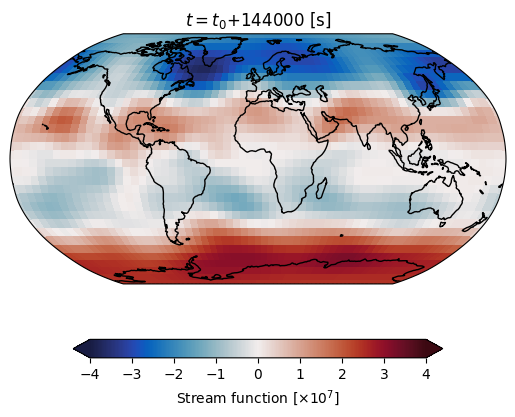
Plot the result
Finally, let us plot the stream function \(\psi\) at the end of the simulation (time = -1) for the first ensemble ensemble member (batch =0). We show only the lowest level (level = -1).
Note that the plot is drawn using matplotlib. We use cartopy to map the latitude-longitude coordinates into the figure for a given projection (ccrs.Robinson here). Also note that we use one of the perceptually uniform colormap from the package cmocean.
[14]:
# TODO: include unit for the stream function
import matplotlib.pyplot as plt
import cartopy.crs as ccrs
import cmocean

fig = plt.figure()
ax = fig.add_subplot(111, projection=ccrs.Robinson())

lon = trajectory_xr.lon.to_numpy()
lat = trajectory_xr.lat.to_numpy()
psi = trajectory_xr.psi.isel(time=-1, batch=0, level=-1).to_numpy() / 1e7
time = trajectory_xr.time.to_numpy()[-1]

ax.set_title(f'$t=t_0$+{time} [s]')
im = ax.pcolormesh(
    lon,
    lat,
    psi,
    cmap=cmocean.cm.balance,
    vmin=-4,
    vmax=4,
    transform=ccrs.PlateCarree(),
)
ax.coastlines()
plt.colorbar(
    im,
    orientation='horizontal',
    extend='both',
    fraction=0.05,
    shrink=0.75,
    label='Stream function [$\\times 10^{7}$]',
)
plt.show()
[ ]: